Datasets come in all forms and shapes. they may contain mistakes, weird formats, etc. So before jumping into the processing of the data we need to make sure that the original dataset is properly set.
This step could be carried out in python, or in any other platform, as you prefer. For example, you may clean your dataset in Excel or SPSS. For this tutorial, we will carry out these operations in Python, but feel free to clean your dataset with other tools and then jump into Python for the next part.
The cleaning steps we should take care are the following:
- Data shape
- Consistency
- (eventual) Binning
- Missing data
1.0. Open the dataset
For cleaning and analyzing our dataset, we will be using Python’s packages Pandas and Numpy (which we will abbreviate in the code as pd and np respectively). Therefore, we run:
import pandas as pd
import numpy as np
If your code is already giving you some errors, it is likely that you do not have these packages installed. To install a package, you can follow this guide here.
Once we have our favourite packages, we can import the file as a dataframe using Pandas.
The first thing you should do is to identify the file extension of the file you want to read. For example, for csv files, you will use the function pd.read_csv(), for excel pd.read_excel(), and for spss pd.read_spss(). You can find the full list of the files you can open here.
The second thing you want to do is to check if there is something weird with the file. For example, if you are using excel, the data you want to open may be in a specific sheet and you should tell this information to python, for example:
pd.read_excel('filename.xlsx', sheet_name='theSheetYouWantToRead')If you are using the manipulated dataset for the tutorial, the csv file may look fine, but if you try to import it, you will find an error:
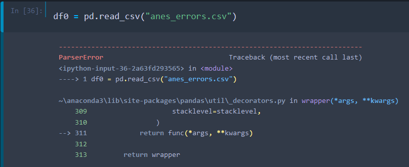
This is because csv format allows for different separators. So, in this case, instead of using the comma, we saved the file using the semicolumn.
Therefore, if you want to open this “dirtied” version of the file, you will need to specify to python that it needs to use the semicolumn as a separator. In the code we can write this as:
df0 = pd.read_csv("anes_errors.csv", sep=';')However, if you are just using the original dataset (which uses the comma as a separator), you can avoid this specification and write:
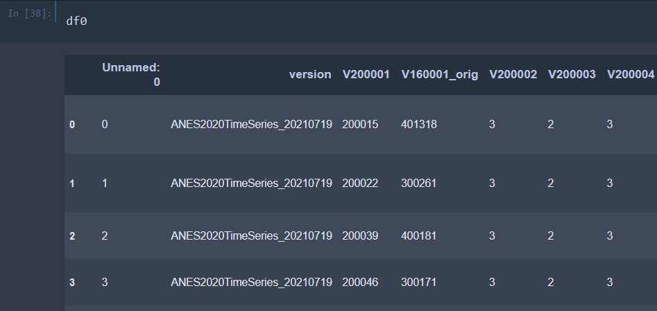
df0 = pd.read_csv("anes_timeseries_2020_csv_20210719.csv")Once you have imported the dataframe into the variable df0, you can print it to make sure that the import went well.
1.1 Data shape
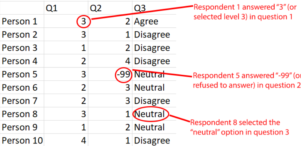
For this tutorial, we will suppose that data is in the shape which is common in many surveys. Meaning that each row will identify a participant and each column an item/question. This does not mean that it is not possible to use ResIN with other data shapes. But to do so, you will probably have to either reshape your data or apply some changes in the code.
Also, since ResIN is quite a flexible method, it will not care if you have numbers and words in the same dataset or even in the same column. This does not matter as ResIN treats each variable as if it was nominal (despite then being able to reconstruct eventual ordinal properties of the data).
Here is a visual example of the data shape you should have and their interpretation.
Notice also that here we are presenting a classical analysis of “respondents” and “responses.” However, Resin can be used to observe even different types of associations.
1.2 Select the variables
1.2.1 Types of variables
There are two type of variables which will be important for making the network: node variables and heat variables. These are informal names to distinguish two types of variables that we will be using for our analysis. Let see what they are.
Node variables are the variables that will produce the nodes of the network. For example, in the network we showed in the last page there were some nodes called gun something. For example “gun:1.0” and “gun:2.0,” etc. This means that these nodes represent different response options (i.e. 1, 2, etc.) of the question on guns. Therefore, the variable gun will be considered as a node variable (as it is used to produce nodes). Note that you cannot produce a network without node variables, so you always have to include some node variables in the analysis.
Heat variables are instead used to produce heatmaps. For example, in the network we showed before, each node has a colour ranging from red to blue. This colour represents the correlation with the rating of Republicans. Meaning that people who selected the red nodes tend to rate Republicans with a bigger score, while people who selected the blue nodes tend to rate Republicans with a lower score. Node variables are not fundamental and you can perform your study also without having them.
In brief, node variables are used to build the network and see how different answers relate to each other (e.g. people who select X tend to select also Y). Instead, heat variables are used to explore if the patterns you observe are connected (or confirmed) by some additional variable.
Notice also that the difference between the two is not due to some kind of inner property. This means that a specific variable will be either a node- or a heat-variable depending on what you would like to explore. Indeed, you could re-run the same analysis including the heat-variable we will use as a network variable.
1.2.2 Setting the variables
In our example, we decided to have 8 node-variables which are 8 political items in the dataset. For example:
V201417: Which [response] comes closest to your view about what government policy should be toward unauthorized immigrants now living in the United States?
While for the heat-variables we decided to have only one. This is the already mentioned rating of the Republican party:
V201157: How would you rate the Republican Party [From 0 to 100]
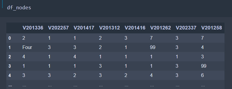
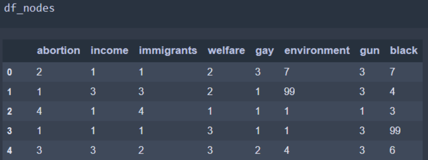
To keep things clean we can create a new dataframe for each type of variables. In this way, each dataset will contain only the variables of interest. Therefore for the nodes we can first select the questions we want to include:
list_of_node_variables = ['V201336', 'V202257', 'V201417', 'V201312', 'V201416', 'V201262', 'V202337', 'V201258']And then create the new dataset containing only these variables:
df_nodes = df0[list_of_node_variables]So, if you now show df_nodes you will see a new dataset containing only the variables we are going to analyze.
We can repeat the same procedure for the heat variables by writing:
list_of_heat_variables = ['V201157']

df_heat = df0[list_of_heat_variables]
Which produces this new dataset with the heat variable(s):
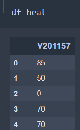
1.3 Labelling consistency
As mentioned before, Resin does not really care about how you label your levels, as long as you are consistent with it.
To give you an example, the European Social Survey asks participants about their positioning on the left-right political spectrum. While positions 1 to 9 are stored in the dataset as numbers, position 0 is stored as “Left” and position 10 as “Right.” Therefore, in the column of this question you will have a mixture of numbers and words.
The thing is: Resin does not really care about this as long as the labelling is consistent. For example, “Left” should be always spelt in the same way.
To give you another example, we can use our “dirtied” dataset. As mentioned, we previously modified entry “V201336.” We can inspect it by typing:
df_nodes["V201336"].unique()The command df0[“V201336”] picks up the column named “V201336” from the dataset df0. Then .unique() collects only its unique elements (i.e. without any repetitions).
The output is the following:
array(['2', 'Four', '4', '1', '3', '4.0', '5', '-9', '-8'], dtype=object)You can note here that there are three similar entries: ‘Four’, ‘4’, and ‘4.0’. While they are the same for a human, ResIN, being a simple algorithm, cannot distinguish between them. Therefore it will consider them as three different values.
Therefore, you will need to clean this and choose a single label for the three of them. Otherwise, Resin will “think” that “Four” and “4.0” are two different answers. Therefore, you will end up with multiple nodes representing the same answer.
In the Jupyter notebook you can clean this just by replacing all the “Four” and “4.0” with “4”.
mask = df_nodes["V201336"]=="Four"
df_nodes.loc[mask, "V201336"] = '4'

mask = df_nodes["V201336"]=="4.0"
df_nodes.loc[mask, "V201336"] = '4'
Where the first line generates a mask (i.e. a series of True and False. True for columns where the value of the columns is “Four” and False otherwise). Then the second line replaces the values of the mask with “4”.
Remember that you do not need to carry out these operations in Python, as you may want to clean your dataset with your favourite software.
1.4 Readability
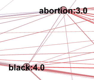
When making the network, Resin will produce nodes which are item-responses (i.e. the answer to a specific question). For example, one node may be immigration:agree. This would be the answer “agree” to the question about “immigration.” For example, in this image, you can see how the third level on abortion is close to the fourth level of a question about black people.
However, nodes will not get readable names magically and if we do not do anything about this, we may end up with nodes named like “V200006:-2” which may be very hard to understand!
For doing so, we need to rename column names (i.e. the questions) in such a way that they can be meaningful. Also, we need to make sure to give them a short name, otherwise visualizing them would be a disaster.
In python we can do this by firstly defining a dictionary containing the old names and the new ones:
dic_nodes = {"V201336":"abortion",  "V202257":"income", "V201417":"immigrants",
     "V201312":"welfare","V201416":"gay","V201262":"environment",
             "V202337":"gun", "V201258":"black"}
Then we run the following command that will replace the names using the previous dictionary:
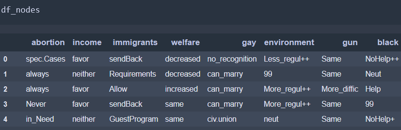
df_nodes = df_nodes.rename(columns=dic_nodes)We can confirm this by showing again the dataframe:
Then we can repeat the same procedure with the heat-variable dataframe:
dic_heat = {"V201157":"ThermoRep"}
df_heat = df_heat.rename(columns=dic_heat)
Finally, you can also rename the responses. For example, instead of using 1.0 you can use “Strongly agree” if this makes sense with your survey. This may help you in better reading the network. Indeed, “immigration:positive” immediately tells us that people who selected that node are positive about immigration. Instead, “immigration:1.0” tells us only that it is the first level of the item, but we do not know if people selecting it are positive or negative about immigration.
In this case we rename each response option, by reading the manual and choosing a short name which can be as meaningful as possible. In python, we ca do this by using a dictionary:
dic_ans = {"abortion":{"1":"Never","2":"spec.Cases","3":"in_Need","4":"always"},
       "income":{"1":"favor","2":"oppose","3":"neither"},
       "immigrants":{"1":"sendBack","2":"GuestProgram","3":"Requirements","4":"Allow"},
       "welfare":{"1":"increased","2":"decreased","3":"same"},
       "gay":{"1":"can_marry","2":"civ.union","3":"no_recognition"},
       "environment":{"1":"More_regul++","2":"More_regul+","3":"More_regul","4":"neut",
                      "5":"Less_regul","6":"Less_regul+","7":"Less_regul++"},
       "gun":{"1":"More_diffic","2":"Easier","3":"Same"},
       "black":{"1":"Help++","2":"Help+","3":"Help","4":"Neut","5":"NoHelp","6":"NoHelp+","7":"NoHelp++"}
          }
Notice also how the ANES dataset sometimes uses a weird coding in which 1 is positive, 2 is negative and 3 is neutral. Therefore, using numeric coding would be much more complex to read.
We can then replace all these values in the dataframe by (1) setting every column as a string with df_nodes[c].astype(str) and then replacing the values using the previous dictionary using df_nodes[c].replace
for c in df_nodes.columns:
    df_nodes[c] = df_nodes[c].astype(str)
    df_nodes[c].replace(dic_ans[c], inplace=True)
Therefore, we end up with the following dataframe:
1.5 Binning (eventually)
As you may have read already, ResIN treats each response option as a nominal variable. Despite this, it is still able to reconstruct the ordinal nature of the data (if it exists), but for doing so it needs multiple people to have selected the same option.
For example, it can “recognize” that the option strongly agree is similar to weakly agree as people who selected the first have a similar response pattern to the people who selected the second. However, to “detect the response pattern of the people who selected strongly agree” we need multiple people to select this option, so that a pattern can appear.
Therefore, if an item has, say 100 levels, it is very likely that we will have only a few people who selected each response option (e.g. even with 1,000 participants we will have on average 10 people per level). This means that we will have a lot of random fluctuations in our data and we may end up just measuring noise (later you will see how to quantify that you are not measuring noise).
Because of that, if a question has a lot of possible responses, it is a good rule to bin it. Meaning that we will merge multiple responses. For example, instead of having responses ranging from 1 to 100 (in steps of 1), we can make them range from 1 to 10 (in steps of 1). Therefore, strongly decreasing the number of levels. You can do it, for example, by turning values 1-10 into 1, 11-20 to 2, etc.
When analyzing the network, you will see some quantitative methods to access if the links are actually statistically significant or if you are analyzing noise. However, if you are starting, let us say that a good rule of thumb is to have ~ 5 levels for each variable.
Note that this applies only to the “node-variables.” While the “heat variables” can have as many levels as you like (even millions if you like to).
Notice that if you already have a reasonably low number of answers you do not need to bin anything. Indeed, also in our example, we do not need to bin the standard values. However, as we will see in a moment, we will have a sort of binning on the missing values.
1.6 Missing values
The last important part of the cleaning process regards the missing or rejected values. Indeed, while many methods ask you to exclude these values from the analysis, ResIN can actually include them. For example, you can leave them in the analysis and find that there is a strong connection between republican attitudes and rejecting some specific questions.
However, you may need to check if your data present different types of missing/rejected data.
For example, in some questions the ANES data distinguishes between ‘Don’t know’ coded as -8 and ‘Refused’ coded as -9. Depending on what you would like to analyze you may want to distinguish between them or not. If they are equivalent for your study, you can merge them choosing a single label for both (i.e. binning them together). Also, you may want to keep only one type (e.g. “Don’t know”) and exclude the other from the analysis. This will depend on what you want to analyze.
For this tutorial, we decided to consider in the same way all the non-standard options. i.e. missing values, refused answers, “don’t know” etc.
For doing so, we use the dictionary of the answers that we built previously and we check if each answer is in the dictionary or not. If not, it will be set to “Ref” which will be our label for the Refused/Missing values. In the code:
for c in df_nodes.columns:
    mask = []
    line = df_nodes[c]
    dic_ = dic_ans[c]
    for el in line:
        val = not (el in dic_.values())
        mask.append(val)
    mask = np.array(mask)
    df_nodes[c][mask]="Ref"
Where, for each column, we build a mask. This mask will be True for the elements of the columns which are not in the dictionary (i.e. non-standard answers) and False otherwise. Then for such a column we replace all these values with “Ref”
And now we are ready for our next step: making the dummy-coded dataframe.