3.1 Working principle
Also the process for making the network is quite straightforward in principle. Later we will see how we can make it much more flexible, but let us start with a heavily simplified version (which will still work).
The general idea is that all the variables in df_nodes will become the nodes (i.e. the dots) of the network. Furthermore, the correlation between them will be the weight of the links. The only additional thing is that negative correlations will be set to zero (at least for this tutorial, as we will explain in a moment, you could actually keep it and re-use it later).
Since this is another step that may generate some questions let us directly address possible misconceptions and problems
q1. Are we losing information… again?
Similarly to our discussion on the previous page, also here we are not really losing information. The “trick” is that the new dataset has a lot of redundancy as each variable has been “expanded” into multiple ones.
To give you an idea that, overall you are gaining and not losing information, consider two variables (e.g. gun control and immigration) each one with 5 possible answers. If you are using a “classical method” you will probably end up with a single number summarizing how strong is the relationship between these two variables (e.g. a correlation coefficient).
ResIN instead will check the correlation between each couple of answers of the two questions (i.e. 25 possible pairs). Even if only 10 of these are positive (therefore we will neglect the 15 negatives) we have 10 numbers (instead of a single one) describing the relationship between these two variables. Therefore, in this example, we end up with “10 times more information” than with a classical method.
q2. Ok, but why not keeping them?
The very short answer is: because negative correlations will not add anything useful/interesting and they will mess things up pretty badly.
If you want to go fully in details, check out this paper. But the main reasons are:
- If you also plot the negative relationship, most likely the network will be so crowded that it will be quite hard to read, nullifying the visual simplicity of ResIN.
- Force-based algorithms (which we will use for locating the position of the nodes) do not work natively with negative edges.
- Negative correlations behave non-linearly respect to the attitude space.
- Removing negative correlations also removes “fake relationship” between answers from the same question (which, being mutually exclusive, will have a negative correlation coefficient).
- Negative correlations contain “bad information.” To be specific, they are insensitive in changes in the attitude space after a certain distance.
- You can still recover all the “important information” (such as ordinality) by using only the positive correlations.
So, yes, negative correlations will require an entirely new algorithm only for dealing with them and they will add pretty much nothing to the analysis.
q3. Does this mean that I will not be able to study negative correlations between variables?
This question may arise when people confuse the original variables (e.g. gun control and immigration) with the dummy-coded variables (e.g. immigration:agree).
If the original variables have a negative correlation, ResIN will simply show to you that immigration:agree correlates with gun control:disagree. If, instead, the original variables are positively correlated immigration:agree will correlate with gun control:agree.
So, yeah, no worries, the correlation between the original variables can be positive or negative without affecting the analysis in any way.
q4. What if I really really want to keep the negative correlations?
In general ResIN does not require removing the negative links. However, getting rid of them can strongly simplify the process at the cost of information that most likely will be useless and that will get in your way while exploring the network.
To keep the negative links several possibilities are available, such as:
- Use the ResIN network without the spatial information (i.e. skipping the force-directed algorithm)
- Use a force-directed algorithm wich ignores the negative edges
- Use a network without the negative edges for finding the nodes’ positions and then including them in the original network having both positive and negative links.
In this tutorial, for simplicity, we will ignore the negative correlations.
3.2 Simplified code
Let us first provide a simplified version of the code. Later, we will show an improved (but more complex) version which will be optimized and will offer much more flexibility.
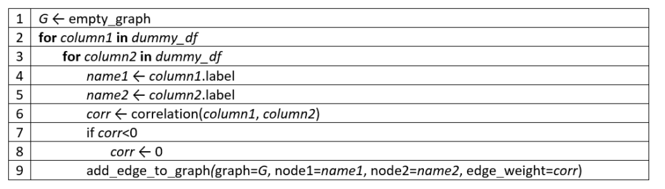
As previously mentioned, the network can be obtained by spanning over each couple of columns and calculating their correlation.
In pseudocode:
In Python, we will start by importing two packages: networkx, which will be used to make the network and scipy.stats which will be used only for calculating the correlation.
import networkx as nx
import scipy.stats as stt
Then we introduce the function make_graph_simplified() which will transform the input (dummy-coded) dataframe into a graph
def make_graph_simplified(df):

    G = nx.Graph()
    list_of_nodes = df.columns

    for node_i in list_of_nodes:
        for node_j in list_of_nodes:

            # Get the two columns
            c1 = df[node_i]
            c2 = df[node_j]

            (r,p) = stt.spearmanr(c1,c2)
            if r<0:
                r = 0

            if r>0:
                G.add_weighted_edges_from([(node_i,node_j,r)],weight='weight')

    return G
Finally, we can just run the function on dummy_df obtaining the network G.
G = make_graph_simplified(df_dummy)Now, if you are in a super rush because you have a presentation in 5 minutes on this method and you remembered to prepare it only now, you can just save your graph file…
filename = 'ANES_simplified'
nx.write_gexf(G,filename+'.gexf')
… and open it with Gephi. If you run it with Force Atlas 2, it will look something like this:
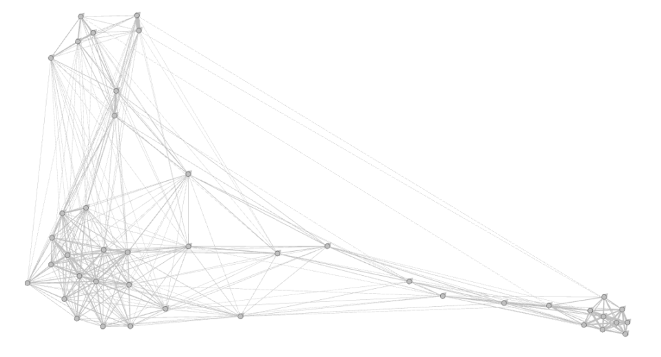
It’s not going to be great, but it definitely looks like something. You should be able to build some kind of narrative around it. Good luck!
However, if you have some extra time, here’s how you can get the maximum out of ResIN.
3.3 A better code for more flexibility
Besides lack of optimization, the previous code had a couple of big limitations:
- Dealing with missing data
- Providing information about p-values
Since on this page we already have a ton of information, we will not discuss the code in detail. Instead, we will just provide the code of the functions and discuss the inputs and outputs.
Therefore, the simplified function make_graph_simplified() is here replaced by the function make_graph_() and its 3 additional functions phi_(), p_val() and phi().
def make_graph_(df, list_of_nodes, alpha=0.05, get_p=True, remove_nan=False, remove_non_significant=False, exclude_same_question=True, print_=False):

    if get_p==False and remove_non_significant==True:
        print("Warning: Setting remove_non_significant to False as get_p is False!")
        remove_non_significant=False

    G = nx.Graph()

    count = 0
    for i, node_i in enumerate(list_of_nodes):
        for j, node_j in enumerate(list_of_nodes):

            if j <= i: # do not run the same couple twice
                continue

            if print_:
                count += 1
                l = len(list_of_nodes)
                n_tot = l*(l-1)/2
                print(count,"/",n_tot, " = ", np.round(count/n_tot,decimals=2)*100, '%')

            basename1 = node_i.split(sep=':')[0]
            basename2 = node_j.split(sep=':')[0]

            if exclude_same_question:
                if basename1 == basename2: # if they belong to the same item
                    continue

            # Get the two columns
            c1 = df[node_i]
            c2 = df[node_j]

            if remove_nan:
                if ("Ref" in node_i) or ("Ref" in node_j):
                    continue

                c1_n = df[basename1+":Ref"] # get the refused values of each item
                c2_n = df[basename2+":Ref"]

                mask = np.logical_not(np.logical_or(c1_n, c2_n)) # get a mask of the refused values

                c1 = c1[mask] # select only the non-nan element
                c2 = c2[mask]

            if get_p:
                (r,p) = phi(c1,c2, get_p=True)
            else:
                r = phi(c1,c2, get_p=False)

            # Check if there are the conditions for drawing a node
            if remove_non_significant:
                condition = r>0 and p<alpha
            else:
                condition = r>0

            if condition:
                G.add_weighted_edges_from([(node_i,node_j,r)],weight='weight')
                if get_p:
                    G.add_weighted_edges_from([(node_i,node_j,p)],weight='p')
                    sig = float(p<alpha) # Boolean are not accepted as edge weight
                    G.add_weighted_edges_from([(node_i,node_j,sig)],weight='sig')
    return G


def phi_(n11,n00,n10,n01):
    n1p = n11+n10
    n0p = n01+n00
    np1 = n01+n11
    np0 = n10+n00

    num = n11*n00-n10*n01
    den_ = n1p*n0p*np0*np1

    if den_==0:
        phi_=np.nan
    else:
        phi_ = num/np.sqrt(den_)
    return phi_


def p_val(r,L):
    den = np.sqrt(1-r**2)
    deg_free = L-2
    if den==0:
        p = 0
    else:
        num = r*np.sqrt(deg_free)
        t = num/den
        p = stt.t.sf(abs(t), df=deg_free)*2
    return p


def phi(x,y,get_p=False):

    m_eq = x==y
    m_diff = np.logical_not(m_eq)

    n11 = float(np.sum(x[m_eq]==True))
    n00 = float(np.sum(x[m_eq]==False))

    n10 = float(np.sum(x[m_diff]==True))
    n01 = float(np.sum(y[m_diff]==True))

    phi_val = phi_(n11,n00,n10,n01)

    if get_p:
        p = p_val(phi_val,len(x))
        return phi_val, p
    else:
        return phi_val
To use it you will have to run:
# Parameters
remove_nan=True
get_p=True
remove_non_significant=False
alpha=0.05

# Get the graph
G = make_graph_(df=df_dummy, list_of_nodes=df_dummy.columns, alpha=alpha, get_p=get_p, remove_non_significant=remove_non_significant,
                remove_nan=remove_nan, exclude_same_question=True, print_=True)
This last block will probably be the only one you will play with as it contains the variables:
- remove_nan
- get_p
- remove_non_significant
- alpha
What do they mean? And what do they do?
remove_nan asks you if you want to keep in the analysis also the missing values (here labeled as “Ref”). If you select False you will also have in your network nodes such as immigrants:Ref, if you select True you will only have non-missing values.
The other three variables regard the p-value of the links. Indeed, as mentioned, the links between nodes are calculated as correlations. However, how do we know if a connection between two nodes is significant or due to noise?
Luckily, correlations allow you to calculate a p-value that can be used to test the significance of each edge. Specifically, get_p asks you if you want to calculate the p-value for each edge. You have the possibility to turn it down as the calculation of the p-value may slow down the process for very big datasets.
alpha is the threshold for the significance test. An alpha of 0.05 means that only p-values below 5% will be considered significant.
Finally, remove_non_significant asks you if you want to remove the edges with non-significant correlations.
We will see a little more about how you can play with these parameters in the final section.